
I like ambient videos to put on the background while doing something else such as bears fishing or train footage going through the Alps or fireflies. It scratches the itch of a screensaver too. Recently I was looking for videos of stars, such as what you’d see from a spaceship. However, I felt like some of them were a bit odd in that they looked “unrealistic”. Not that I’d been on a starship before, but somehow the distribution of stars seemed off. Maybe not enough diversity in brightness and size, or maybe the density was not quite right. It really felt artificial in that the same code that generated the stars could have been used to generate falling snow or at the very least was some kind of too-uniform distribution of random positions. That made me think:
If generating stars belonging to some uniform distribution is unrealistic, what would be a better function to use? So I looked it up, had a couple of arguments with my local LLM, and found out that it does exist and it’s called an Initial Mass Function or Stellar Mass Function. That seems to be exactly what I was looking for – if a random set of stars looks unrealistic, then surely it has something to do with the randomness function used. Unfortunately, the universe itself is quite complex and comprises of multiple different substructures such as galaxies and globular clusters so it’s not like a simple analytical function can cover the whole range, but at least maybe I can start with those substructures.
Turns out this is pretty well studied and the first model describing this structure is the King model and look there’s even a python package for this stuff! So we get the PDF of the cluster:
from limepy import limepy
import numpy as np
import matplotlib.pyplot as plt

plt.style.use("dark_background")

k = limepy(7, 1)

fig, ax = plt.subplots()
ax.plot(k.rho, k.r)
ax.set_xlabel("rho")
ax.set_ylabel("r")
plt.savefig("king.svg")and we can then generate a nice cluster:
cdf = np.cumsum(k.rho)/np.sum(k.rho)

N = 10000
r = np.interp(np.random.uniform(0,1,10000), cdf, k.r)
phi = np.random.uniform(0,1,N) * 2 * np.pi

x = r * np.cos(phi)
y = r * np.sin(phi)

fig, ax = plt.subplots(figsize=(10,10))
ax.set_aspect("equal")
ax.set_frame_on(False)
ax.scatter(x, y, s=1, color="white");
ax.set_xticks([])
ax.set_yticks([])
plt.savefig("cluster.svg", bbox_inches="tight", pad_inches=0)
Neat! Looks reasonable but not sufficient yet. Perhaps we need to model some more complex structures? More on that in a bit but while reading about globular clusters I learned about how useful they were in defining our position in the galaxy. Since the galaxy appears as dense (in terms of number of stars, or their implied distance by brightness) on either side of the celestial sphere, we assumed that we had to be near the center of the galaxy.
Turns out that this is highly skewed by interstellar dust which naturally puts us at the center of our own limited visibility area. However, as globular clusters are spherically distributed around the galaxy, thus less affected by dust, our measurements of distance and density for those are not skewed. Based on those measurements, we were able to determine our distance from the center of the galaxy. I probably butchered the explanation so here are some more sources on this:
Okay, now back to:
Now those are way prettier but unlike the globular clusters, galaxies are not simply described by a 1-dimensional density function that simply relies on the distance from the center. While we still model their mass density (and subsequently their potential field) with a similar distance-based function, the resulting spiral shape is best described as an artifact of the shape of orbits.
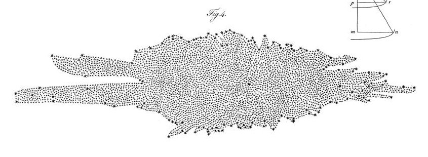
The specific theory describing the characteristic spiral shape is Density wave theory. Looking at the graph on Wikipedia we get a quick idea of what it suggests:

Okay so that looks like stars follow elliptical orbits around the black hole at the center, each orbit having its long axis slightly offset, and the orbits form a “density wave” or “traffic jam” at the regions where they are closest, which has this spiral structure. Elliptical orbits sound reasonable at first since I remember Kepler`s first law from some physics class a decade ago… but no! Kepler’s first law states that the orbit is elliptical with the black hole at one of the foci and not at the center! So what kind of weird orbits are these? From Frank Shu’s review titled Six Decades of Spiral Density Wave Theory
Suppose that there was a force that perturbed the orbits of stars away from mean shapes that are circles. In an inertial frame, each star would follow a perturbed epicyclic path that would not close in a frame with zero angular speed. But in a frame that rotated at some pattern speed Ωp, the orbits might close, with a generic shape easiest to imagine (with a kinematic basis in Bertil Lindblad’s theory of epicyclic orbits in an axisymmetric force field) having a two-lobed oval. … It was C.C. Lin’s insight, after viewing Per Olof Lindblad’s early N-body simulations of the phenomenon, that perhaps the nonaxisymmetric force associated with the self-gravity of the spiral distribution of the surface density would allow the Ωp, which closes the orbits, to have the same value at all ϖ.
Ah! that makes much more sense. So if I got that right: 1. These shapes are not necessarily ellipses, but perturbed circles or two-lobed ovals 2. The potential field of the galaxy is special such that the equipotential orbits are not circular 3. The disk rotates at a constant pattern speed Ωp at all radii, which introduces the phases of the orbits
Ok so to plot that we assume that in polar coordinates our orbits are R(t), Phi(t) with R(t) = r + ε(t) and Phi(t) = Ω . t + θ(t) . t where ε and θ are the off-circle deviations, Ω is the inertial frame rotation speed and r is the corresponding circle radius. We express the radius deviation as: ε(t) = A . r . cos( κ . t + φ0 ) and by conservation of angular momentum we get that φ(t) = -2 . Ω . A / κ . sin( κ . t + φ0 ) (see here for some more in-depth derivations).
A lot of the free parameters here are actually meaningful in real galaxies and are derived from the actual modeled potential, but here we just want to draw some pretty plots so I guessed at parameters until I got some pretty plots:
import matplotlib.pyplot as plt
import numpy as np

plt.style.use('dark_background')

fig,ax = plt.subplots(figsize=(10,10))
ax.set_frame_on(False)
ax.set_aspect('equal')

Omega_p = 30
A = 0.08
spirals = 2

for i,r in enumerate(np.arange(0.2,10,2*A)):
    kappa = 10 + r
    phi0 =  r * 20 * A

    t = np.arange(0,np.pi*2,0.1/kappa)

    Omega = Omega_p - kappa/spirals
    R = r + A * r * np.cos( kappa * t + phi0 )
    Phi = Omega * t - 2 * Omega * A / kappa * np.sin( kappa * t + phi0 )
    Theta = Phi - Omega_p * t

    x = R * np.cos(Theta)
    y = R * np.sin(Theta)

    ax.plot(x, y, color="white")

ax.set_xticks([])
ax.set_yticks([])
plt.savefig("orbits.svg", bbox_inches='tight', pad_inches=0)
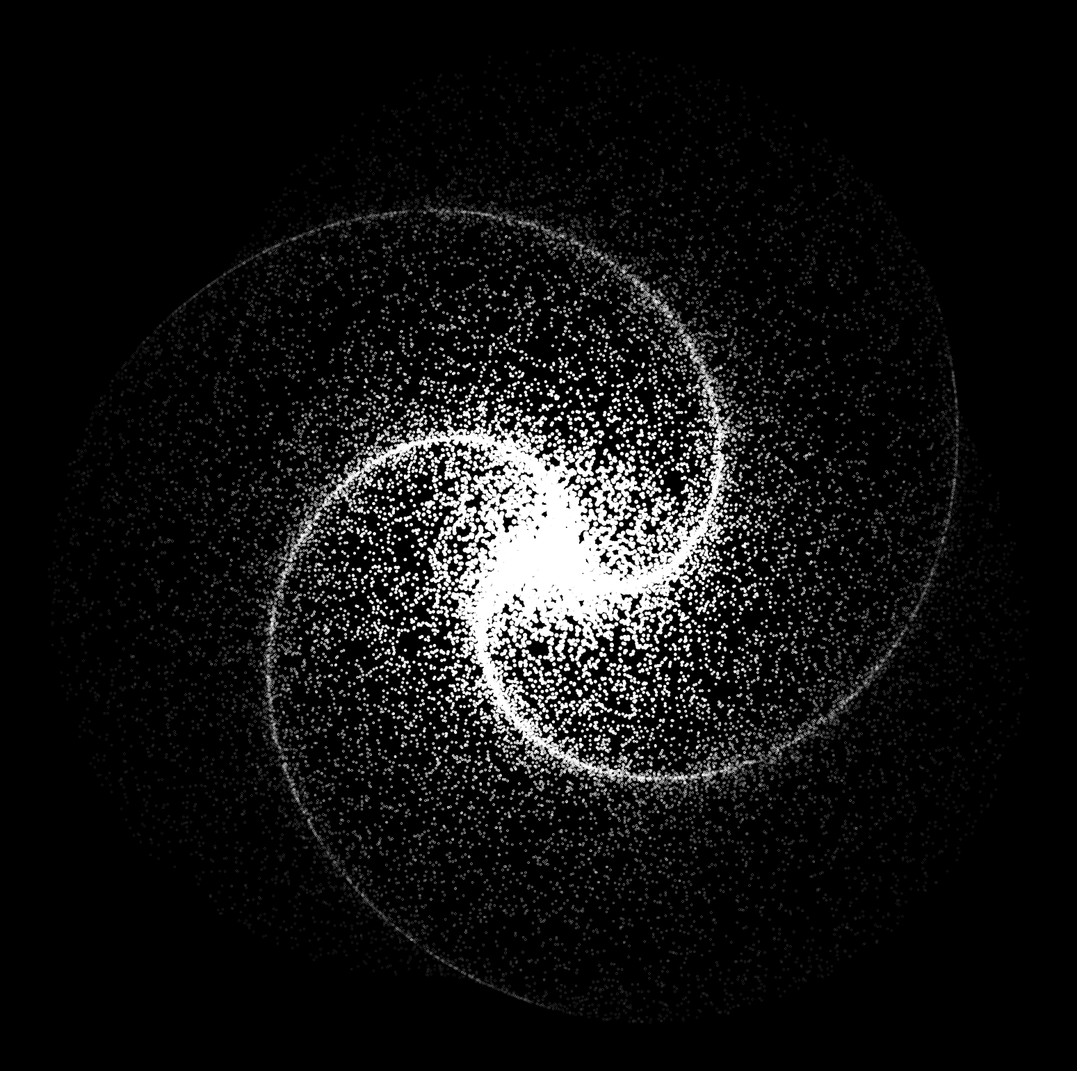
And with some more guessing on the brightness/density curve we can sample points along those orbits:
fig,ax = plt.subplots(figsize=(10,10),dpi=200)
ax.set_frame_on(False)
ax.set_aspect('equal')

N=30000

r = np.random.uniform(0, 10, N)
t = np.random.uniform(0, np.pi*2, N)

kappa = 10 + r
phi0 =  r * 13 * A

Omega = Omega_p - kappa/spirals
R = r + A * r * np.cos( kappa * t + phi0 )
Phi = Omega * t - 2 * Omega * A / kappa * np.sin( kappa * t + phi0 )
Theta = Phi - Omega_p * t

x = R * np.cos(Theta)
y = R * np.sin(Theta)
s = np.exp(-r*0.9+2)

ax.scatter(x, y, color="white", s=s)

ax.set_xticks([])
ax.set_yticks([])
plt.savefig("galaxy.png", bbox_inches='tight', pad_inches=0)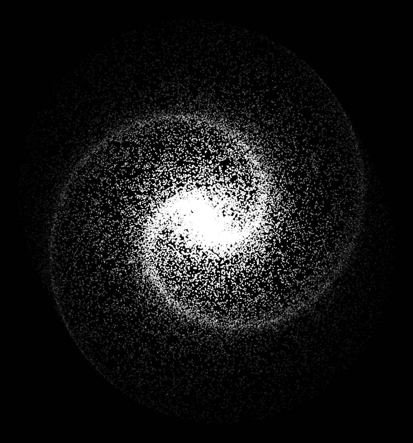
I was a bit dissatisfied with the svg scatterplot because it was not producing regular svg circles so I plotted the svg by hand:
W = 1800
H = 1800
with open("galaxy.svg", "w") as f:
    f.write('<?xml version="1.0" standalone="no"?>')
    f.write('<svg width="{W}" height="{H}" version="1.1" xmlns="http://www.w3.org/2000/svg">'.format(W=W, H=H))
    f.write('<rect x="0" y="0" width="{W}" height="{H}" fill="black"/>'.format(W=W, H=H))
    for i in range(N):
        f.write('<circle cx="{x:.2f}" cy="{y:.2f}" r="{s:.2f}" stroke="white" fill="white" stroke-width="1"/>'.format(x=W/2+75*x[i],y=H/2-75*y[i],s=s[i]**.5 * 2))

    f.write('</svg>')
The neat part is that we can also expand to 3 or more spiral arms here:

While the above are neat and all, we’re still far from something that looks real. Sure the galaxy generation could be better if we take into account the density distribution of the bulge, halo, and disc, but even then, I want something that fills up the field of view. Looking further for more complete models of the galaxy I came across TRILEGAL and Besançon. To my understanding, these are built by fitting an ensemble of specific functions modeling various aspect of the galaxy, such as the Initial Mass Function, a disc mass decay, a model of light extinction due to interstellar dust, and so on. This however is way beyond what I’d be willing to implement. But these models have to be fit on real observational data as they have numerous free parameters which lead me to finding out that:
The European Space Agency has kindly released a huge star survey. This survey tracked locations of stars using an optical telescope at various points during the Earth’s trajectory around the Sun, allowing it to measure the parallax of each light source, which can be used to measure its distance from the solar system. Downloading the survey is pretty straightforward, there is an API but the easiest way I found was to fetch the full files from storage. The full archive is about 730GB of compressed CSV files but after subsetting to just the data we care about and using a slightly better data format can store the universe in 46GB.
We subset each file to just our columns of interest, and store as parquet:
import sys
import pandas as pd

fname = sys.argv[1]
cols = ["ra", "dec", "parallax", "parallax_error", "phot_g_mean_mag", "phot_bp_mean_mag", "phot_rp_mean_mag"]
df = pd.read_csv(fname, usecols=["source_id"] + cols, dtype={"source_id": "int64"} | {k:'float32' for k in cols}, index_col="source_id")
df.to_parquet(fname.replace(".csv", ".parquet").replace("/tmp", "data"), compression='zstd')
and then some plumbing:
curl -s "https://gaia.eu-1.cdn77-storage.com/?prefix=Gaia/gdr3/gaia_source/&delimiter=/" > /tmp/index.xml
URLS=$(xq -r '.ListBucketResult.Contents.[].Key' /tmp/index.xml | sed 's|^|https://cdn.gea.esac.esa.int/&|' )
marker=$(xq -r '.ListBucketResult.NextMarker' /tmp/index.xml)
curl -s "https://gaia.eu-1.cdn77-storage.com/?prefix=Gaia/gdr3/gaia_source/&delimiter=/&marker=$marker" > /tmp/index.xml
URLS="$URLS $(xq -r '.ListBucketResult.Contents.[].Key' /tmp/index.xml | sed 's|^|https://cdn.gea.esac.esa.int/&|' )"
marker=$(xq -r '.ListBucketResult.NextMarker' /tmp/index.xml)
curl -s "https://gaia.eu-1.cdn77-storage.com/?prefix=Gaia/gdr3/gaia_source/&delimiter=/&marker=$marker" > /tmp/index.xml
URLS="$URLS $(xq -r '.ListBucketResult.Contents.[].Key' /tmp/index.xml | grep -v MD5 | sed 's|^|https://cdn.gea.esac.esa.int/&|' )"
rm /tmp/index.xml

function download() {
    fname="/tmp/$(basename $url)"
    fname_decomp=$(echo "$fname" | sed 's/.gz$//')
    fname_final=$(echo "$fname" | sed -e 's/.csv.gz$/.parquet/' -e 's:^/tmp:data:')
    if [ -e "$fname_final" ]; then
        return
    fi
    echo "Creating $fname_final..."
    wget -q "$1" -O "$fname"
    zcat "$fname" | grep -v "^#" > "$fname_decomp"
    rm "$fname"
    python compress.py "$fname_decomp"
    rm "$fname_decomp"
}

cnt=0

for url in $URLS; do
    if (( cnt < 16 )); then
        cnt=$((cnt+1))
    else
        wait -n
    fi
    download "$url" &
done
wait
After waiting a few hours for the data to download, I lift my laptop with one arm. It is no heavier despite containing the firmament.
With the universe at my fingertips I have to construct a simulacrum telescope in order to be able to see it. I project the celestial coordinate angles (right ascension and declination) onto an imaginary plane, scaled by the field of view:
def gnomonic(ra, dec, fov):
    import numpy as np
    x = -np.tan(np.radians(ra))/(2*np.tan(np.radians(fov)))
    y = np.tan(np.radians(dec))/(2*np.tan(np.radians(fov)))
    return x,y
And I turn to Orion’s belt
ra0 = 85
dec0 = 5
df["x"], df["y"] = gnomonic(df["ra"] - ra0, df["dec"] - dec0, 10)
df["s"] = 10**(2-0.5*df["phot_g_mean_mag"])
df = df.query("(x>-1) & (x<1) & (y>-1) & (y<1)")

fig, ax = plt.subplots(figsize=(10,10))
ax.set_frame_on(False)
ax.set_aspect('equal')
ax.set_facecolor("black")
df.plot.scatter(x="x", y="y", s="s", c="white", ax=ax)
I can sort of see Orion here but several stars appear to be missing. It turns out that Gaia did not capture the brightest of stars. Some more data searching later, loading the Hipparcos dataset and merging it in, we see the old familiar sight:
